Modeling the Transfer Market — One Move, Two Rows, and a Fee That Might Not Exist
Most of our dimensional model is about what happens on the pitch — matches, appearances, cards, goals. Adding the transfer market was the first time we modelled a business process that happens off the pitch, and it turned out to be the hardest modelling exercise in the whole project. A transfer looks simple — Player X moves from Club A to Club B for €Y — but almost every part of that sentence has an edge case hiding in it.
That’s the thing about data modelling that’s easy to underrate: the difficulty is almost never the SQL. It’s the decisions. What is the grain? What does a missing value mean? Which entity is this, really, or is it the same entity wearing a different hat? Each of those questions has several defensible answers, and you usually can’t tell which one was right until weeks later, when you’re building a dashboard on top and the model either bends to the question being asked or fights you the whole way. Every modelling choice in this post showed up again downstream — sometimes as a feature that fell out for free, sometimes as a bullet we’d dodged. This post walks through the full journey, from the raw API rows to a fct_team_transfers fact table and the Transfer Intelligence page it powers, and tries to be honest about how often “the modelling” was the work.
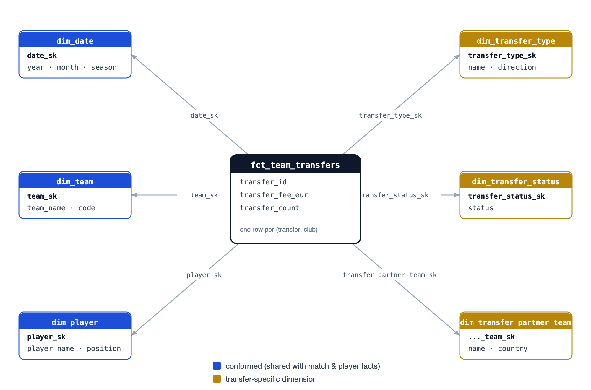
Here’s the model we’re building toward — a classic star schema. fct_team_transfers sits in the centre, joined to six dimensions: three conformed (blue — the same dim_date, dim_team, dim_player the match and player facts use) and three transfer-specific (gold). The rest of this post is the story of how each of those pieces was decided.
The raw shape
Sportmonks gives us one row per transfer, with the player, both clubs, the type, and the fee embedded as nested objects. The silver model flattens that into typed columns:
SELECT
    id,
    player_id,
    from_team_id,
    to_team_id,
    transfer_date,
    career_ended,        -- the player retired instead of moving
    completed,           -- deal done vs still pending
    amount,              -- the fee, in euros — often NULL
    from_team_placeholder,
    to_team_placeholder,
    type_name,           -- 'Transfer', 'Free Transfer', 'Loan', 'End of loan'
    ...
FROM bronze.sportmonks__transfers
Three things in that list caused all the downstream design decisions:
amountis frequently NULL. Sometimes that means “free”, sometimes it means “fee undisclosed”. Those are not the same thing, and conflating them would quietly corrupt every spend metric.- The counterparty club is often not one of our clubs. A Danish club selling to a German one — the German club is foreign and isn’t in our
dim_team. Sometimes it’s aplaceholder(a stand-in for “some club, details unknown”). career_endedtransfers have no destination at all. A retirement is modelled as a transfer with no realto_team.
The grain question: one move, two rows
The hardest decision was the grain. A transfer is fundamentally about two clubs, but a dashboard almost always looks at the market from one club’s point of view — what did FC Copenhagen spend, who did Brøndby sell. We’d already solved this exact shape once, with fct_team_matches: a fixture involves two teams, and we store it as two rows, one per side.
So we used the same pattern. The grain of fct_team_transfers is one row per (transfer, club):
- A normal two-club move emits two rows — the selling club gets an
Outgoingrow, the buying club gets anIncomingrow. - A move where only one side is a club we track (a foreign sale, or a placeholder counterparty) emits only that one real side.
- A retirement emits a single
Outgoingrow for the club losing the player, with no destination.
The model builds this as an outgoing CTE (subject = from_team) and an incoming CTE (subject = to_team), each filtered to rows where its own side is a real, non-placeholder club, then UNION ALL-ed together. The “other” club becomes a partner attribute on the row, not a second subject.
This is the clearest example of a modelling choice paying off downstream. Because the grain is already “per club”, every dashboard query is a plain GROUP BY club — net spend, busiest clubs, incoming vs outgoing — with no self-joins and no “is this club the buyer or the seller?” gymnastics in the SQL. Had we stored one row per transfer with buyer and seller columns instead, every single club-level chart would have needed to UNION the two sides back apart at query time, in the dashboard, repeatedly. We paid that cost once, in the model, where it belongs.
Direction and mechanism in one mini-dimension
Every transfer row needs to answer two questions: which way did the player move (in or out), and how (permanent, free, loan, loan return, retirement). Those are correlated — a “Loan In” is the incoming face of the same mechanism as a “Loan Out” — so we folded them into a single small dim_transfer_type:
SELECT 1 AS transfer_type_sk, 'Permanent Signing'    AS transfer_type_name, 'Incoming' AS transfer_direction
UNION ALL SELECT 2, 'Permanent Sale',      'Outgoing'
UNION ALL SELECT 3, 'Free Signing',        'Incoming'
UNION ALL SELECT 4, 'Free Departure',      'Outgoing'
UNION ALL SELECT 5, 'Loan In',             'Incoming'
UNION ALL SELECT 6, 'Loan Out',            'Outgoing'
UNION ALL SELECT 7, 'Returning from Loan', 'Incoming'
UNION ALL SELECT 8, 'Loan Spell Ended',    'Outgoing'
UNION ALL SELECT 9, 'Retirement',          'Outgoing'
UNION ALL SELECT -1, 'Unknown',            'Unknown'
UNION ALL SELECT -2, 'Not Applicable',     'Not Applicable'
The fact table assigns the surrogate key with a CASE on the raw type_name, choosing the incoming or outgoing variant depending on which CTE it’s in. The same source type — “Loan” — becomes SK 5 in the incoming CTE and SK 6 in the outgoing one. Keeping direction and mechanism in one conformed dimension means a filter like “show me all loan activity” is a single predicate, and the dashboard’s Direction filter is just transfer_direction.
The fee that might not exist
This is the subtlety we’re proudest of getting right. amount is NULL far more often than it’s populated, and there are genuinely three different cases hiding behind that:
CASE
    WHEN amount IS NOT NULL                          THEN amount  -- disclosed fee
    WHEN type_name = 'Transfer' AND NOT career_ended THEN NULL     -- permanent move, fee undisclosed
    ELSE 0                                                         -- free / loan / loan return / retirement: structurally no fee
END AS transfer_fee_eur
A free transfer has a fee of exactly 0. A permanent sale with an undisclosed fee has a fee of NULL — we know money changed hands, we just don’t know how much. Collapsing those two into “0” would understate spend and inflate the count of “free” deals. Keeping NULL distinct from 0 is what lets the dashboard honestly say “Fees shown where disclosed” and report a separate Fee Disclosed Deals count — the number of moves where a real fee was actually published — alongside the total deal count.
The partner club: a role-playing dimension
The other club in a move isn’t a new entity — it’s a club, same as any other, just playing a different role. So dim_transfer_partner_team is a view over dim_team, exactly parallel to how dim_opponent_team is a role-playing view for fixtures:
SELECT
    team_sk      AS transfer_partner_team_sk,
    team_id      AS transfer_partner_team_id,
    team_name    AS transfer_partner_team_name,
    team_country AS transfer_partner_team_country,
    team_logo    AS transfer_partner_team_logo
FROM dim_team
When the counterparty is foreign or a placeholder, the join misses and we fall back to a sentinel key (-1 Unknown). That’s expected and allowed — more on that below.
Conformed dimensions: why a new fact was cheap to add
Here’s the part that made adding an entirely new business process feel almost easy, and it’s worth dwelling on because it’s the whole point of dimensional modelling. fct_team_transfers didn’t need a new calendar, a new club list, or a new player registry. It reused the conformed dimensions that already existed for matches and appearances: the same dim_date, the same dim_team, the same dim_player. A conformed dimension is one that means exactly the same thing — same keys, same attributes — to every fact that touches it. That shared meaning is what lets two facts built months apart talk to each other.
The payoff is concrete and it’s mostly a downstream payoff:
- Because transfers join the same
dim_dateas matches, the dashboard’s Year filter and the derived season logic work identically on the Transfer page as on every other page. No new date handling, no parallel “transfer calendar”. - Because the subject club is the same
dim_teamused league-wide, a club is the same entity on the Transfer page as on its team page — same surrogate key, same name, same logo. Thedim_transfer_partner_teamrole-play sits on top of that same dimension, so a partner club and a “real” club are guaranteed to reconcile. - The only genuinely new dimensions were the two tiny transfer-specific ones (
dim_transfer_type,dim_transfer_status). Everything else was already conformed and waiting.
We keep a bus matrix in the project README — a grid of business processes against dimensions — and adding transfers was, almost literally, adding one column to that grid and ticking the dimensions it shares. When the matrix lines up, a “new” fact is a small, well-understood piece of work. When it doesn’t, you discover that two teams of the same name have different keys in different tables, and integration becomes a debugging nightmare. The boring discipline of conforming dimensions early is what kept this one boring.
Why we rebuild the whole table every run
Every other fact table is incremental on a date window: new matches land, we process the new dates. Transfers break that assumption. A transfer’s effective date has nothing to do with when it shows up in the API — backfills arrive late, and future-dated deals (a summer signing announced in spring) would be skipped entirely by a “process yesterday’s dates” filter. The table is also tiny — on the order of 10k rows. So fct_team_transfers is a plain full rebuild each run. Correct and simpler; the incremental machinery would have been complexity with no payoff.
Tests that encode the weirdness
The edge cases are exactly the things worth testing. Two custom tests guard the model:
- A transfer can’t be between a club and itself. Both sides may legitimately be NULL (counterparty out of scope), so the test only flags rows where both sides are set and equal.
- FK integrity, with deliberate exceptions. The subject club, the type, and the status must always resolve to a real dimension row — a
-1there means a real bug. Buttransfer_partner_team_sk,player_sk, anddate_skare allowed to be-1/-2: an unknown foreign counterparty, an un-ingested player, or a date outsidedim_date’s range are all valid states, not failures. Encoding which sentinels are acceptable and which aren’t is half the value of the test.
From gold to the dashboard
The dashboard reads from a mart_club_transfer_log view that joins everything out and adds one more rule: a club only appears for years it actually played a league match that calendar year. Without it, relegated or not-yet-promoted clubs would show stray transfer rows for seasons they weren’t in the league.
On top of that fact, the Transfer Intelligence page derives a few things that don’t exist in the source at all:
- Transfer windows. Football has registration windows, but the API just gives dates. We derive a
transfer_windowfrom the month — Summer (Jun–Sep), Winter (Dec–Feb), and Outside for everything else. The two main windows capture ~95% of all activity; the rest are free agents, loan returns, and contract terminations that can happen year-round, so an explicit “Outside” bucket keeps them visible instead of dropping them. - Net spend. Per club, fees on incoming moves (Spent) minus fees on outgoing moves (Received) gives Net Spend — positive for net buyers, negative for net sellers — while Transfer Volume (Spent + Received) ranks the clubs moving the most money in either direction.
What we took away
Two things stuck with us. The first: NULL is information. A missing fee, a missing counterparty, a retirement with no destination — each NULL meant something specific, and the model’s job was to preserve those distinctions rather than flatten them into a convenient default. The real work was never the SQL; it was the unglamorous CASE statements that decide whether a blank fee is a zero or an unknown.
The second, and the one we’d put first if we could only keep one: the model is where you win or lose the dashboard. Every hard decision here — the per-club grain, the disclosed/undisclosed/zero fee split, conforming the date, team, and player dimensions — was made days or weeks before anyone built a chart, and every one of them either handed the dashboard a feature for free or quietly removed a class of bug it would otherwise have hit. That’s the uncomfortable, motivating truth of data modelling: the choices are hardest to make exactly when you have the least information about how they’ll be used, and they’re the choices you can least afford to get wrong. Get the model right and the dashboard almost builds itself, honestly. Get it wrong and no amount of clever front-end SQL will stop it lying confidently.